

 Picture by Writer
Correct predictions allow studios to make well-informed choices about varied features, equivalent to advertising, distribution, and content material creation.
Better of all, these predictions might help maximize income and reduce losses by optimizing the allocation of sources.
Luckily, machine studying methods present a strong software to sort out this complicated downside. Little doubt about it, by leveraging data-driven insights, studios can considerably enhance their decision-making course of.
This information science mission has been used as a take-home project within the recruitment course of at Meta (Fb). On this take-home project, we’ll uncover how Rotten Tomatoes is making labeling as ‘Rotten’, ‘Recent’ or ‘Licensed Recent’.
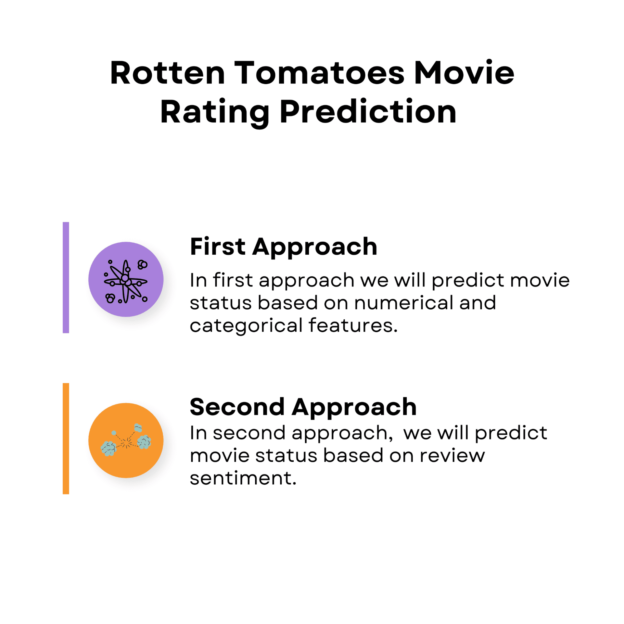
To do this, we’ll develop two completely different approaches.
Picture by Writer
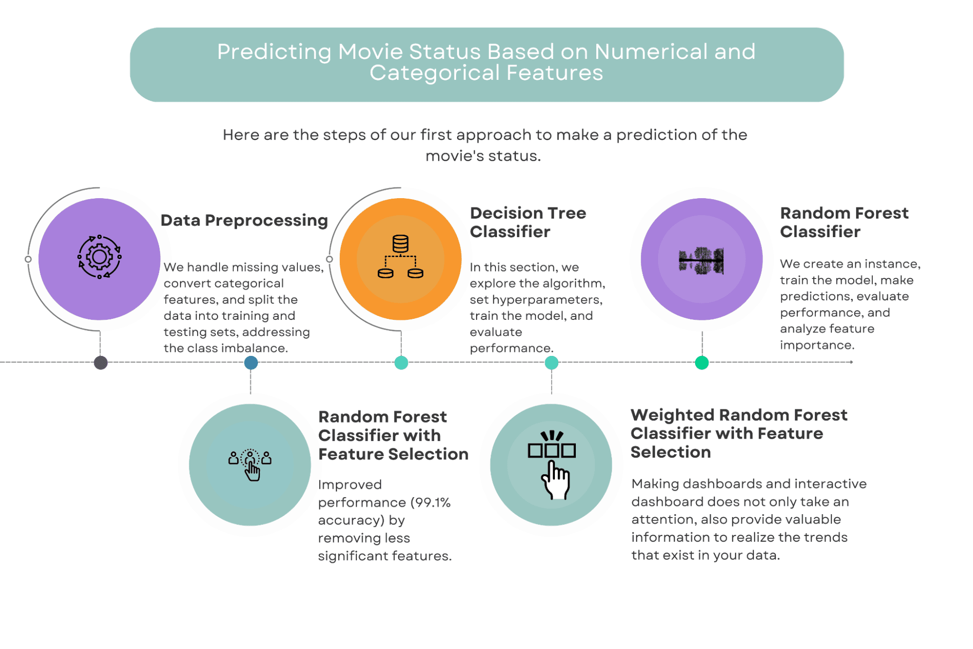
All through our exploration, we’ll talk about information preprocessing, varied classifiers, and potential enhancements to reinforce the efficiency of our fashions.
By the top of this submit, you should have gained an understanding of how machine studying might be employed to foretell film success and the way this information might be utilized within the leisure business.
However earlier than going deeper, let’s uncover the info we’ll work on.

On this method, we’ll use a mix of numerical and categorical options to foretell the success of a film.
The options we’ll think about embody elements equivalent to finances, style, runtime, and director, amongst others.
We are going to make use of a number of machine studying algorithms to construct our fashions, together with Resolution Bushes, Random Forests, and Weighted Random Forests with function choice.
Picture by Writer
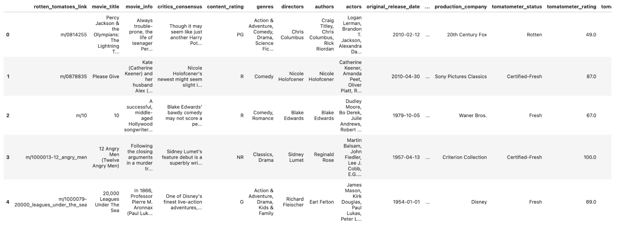
Let’s learn our information and take a glimpse of it.
Right here is the code.
<code>df_movie = pd.read_csv('rotten_tomatoes_movies.csv')
df_movie.head()</code>
Right here is the output.
Now, let’s begin with Information Preprocessing.
There are lots of columns in our Information set.
Let’s see.
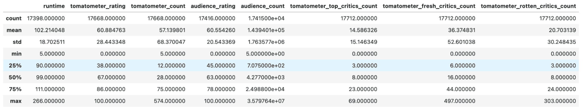
To develop a greater understanding of the statistical options, let’s use describe the () technique. Right here is the code.
Right here is the output.
Now, we’ve a fast overview of our information, let’s go to the preprocessing stage.
Information Preprocessing
Earlier than we will start constructing our fashions, it is important to preprocess our information.
This entails cleansing the info by dealing with categorical options and changing them into numerical representations, and scaling the info to make sure that all options have equal significance.
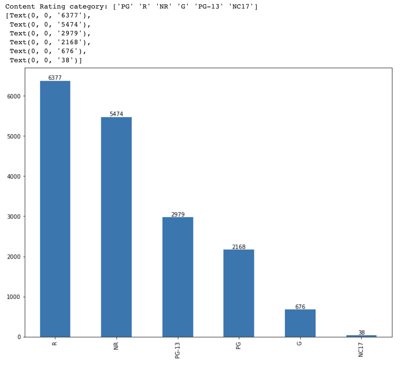
We first examined the content_rating column to see the distinctive classes and their distribution within the dataset.
<code>print(f'Content material Ranking class: {df_movie.content_rating.distinctive()}')</code>
Then, we’ll create a bar plot to see the distribution of every content material score class.
<code>ax = df_movie.content_rating.value_counts().plot(variety='bar', figsize=(12,9))
ax.bar_label(ax.containers[0])</code>
Right here is the total code.
<code>print(f'Content material Ranking class: {df_movie.content_rating.distinctive()}')
ax = df_movie.content_rating.value_counts().plot(variety='bar', figsize=(12,9))
ax.bar_label(ax.containers[0])</code>
Right here is the output.
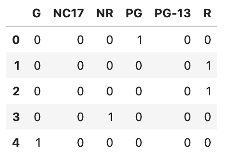
It’s important to transform categorical options into numeric varieties for our machine studying fashions which want numeric inputs. For a number of parts on this information science mission, we’re going to apply two usually accepted strategies: ordinal encoding and one-hot encoding. Ordinal encoding is healthier when classes indicate a level of depth, however the one-hot encoding is good when no magnitude illustration is supplied. For the “content_rating” belongings, we’ll use a one-hot encoding technique.
Right here is the code.
<code>content_rating = pd.get_dummies(df_movie.content_rating)
content_rating.head()</code>
Right here is the output.
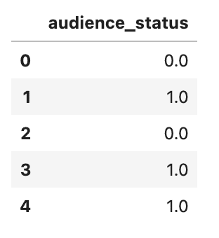
Let’s go forward and course of one other function, audience_status.
This variable has two choices: ‘Spilled’ and ‘Upright’.
We did already apply one scorching coding, so now it’s time to remodel this categorical variable right into a numerical one through the use of ordinal encoding.
As a result of every class illustrates an order of magnitude, we’ll remodel these into numerical values through the use of ordinal encoding.
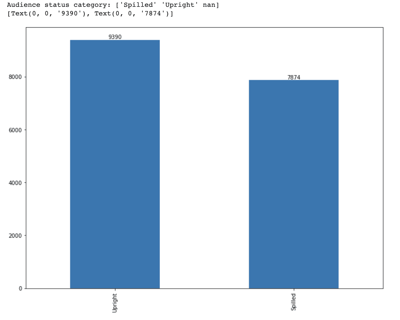
As we did earlier, first let’s discover the distinctive viewers standing.
<code>print(f'Viewers standing class: {df_movie.audience_status.distinctive()}')</code>
Then, let’s create a bar plot and print out the values on prime of bars.
<code># Visualize the distribution of every class
ax = df_movie.audience_status.value_counts().plot(variety='bar', figsize=(12,9))
ax.bar_label(ax.containers[0])</code>
Right here is the total code.
<code>print(f'Viewers standing class: {df_movie.audience_status.distinctive()}')
# Visualize the distribution of every class
ax = df_movie.audience_status.value_counts().plot(variety='bar', figsize=(12,9))
ax.bar_label(ax.containers[0])</code>
Right here is the output.
Okay, now it’s time to do ordinal coding through the use of exchange technique.
Then let’s view the primary 5 rows through the use of the top() technique.
Right here is the code.
<code># Encode viewers standing variable with ordinal encoding
audience_status = pd.DataFrame(df_movie.audience_status.exchange(['Spilled','Upright'],[0,1]))
audience_status.head()</code>
Right here is the output.
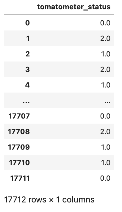
Since our goal variable, tomatometer_status, have three distinct classes, ‘Rotten’, ‘Recent’, and ‘Licensed-Recent’, these classes additionally signify an order of magnitude.
That’s why we once more will do ordinal encoding to remodel these categorical variables into numerical variables.
Right here is the code.
<code># Encode tomatometer standing variable with ordinal encoding
tomatometer_status = pd.DataFrame(df_movie.tomatometer_status.exchange(['Rotten','Fresh','Certified-Fresh'],[0,1,2]))
tomatometer_status</code>
Right here is the output.
After altering categorial to numerical, it’s now time to mix the 2 information frames. We’ll use Pandas pd.concat() perform for this, and the dropna() technique to take away rows with lacking values throughout all columns.
Following that, we’ll use the top perform to take a look at the freshly shaped DataFrame.
Right here is the code.
<code>df_feature = pd.concat([df_movie[['runtime', 'tomatometer_rating', 'tomatometer_count', 'audience_rating', 'audience_count', 'tomatometer_top_critics_count', 'tomatometer_fresh_critics_count', 'tomatometer_rotten_critics_count']], content_rating, audience_status, tomatometer_status], axis=1).dropna()
df_feature.head()</code>
Right here is the output.

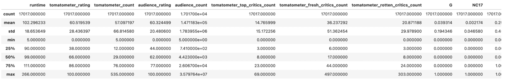
Nice, now let’s examine our numerical variables through the use of describe technique.
Right here is the code.
Right here is the output.
Now let’s examine the size of our DataFrame through the use of len technique.
Right here is the code.
Right here is the output.
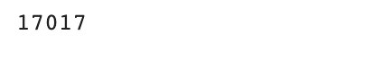
After eradicating rows with lacking values and doing the transformation for constructing machine studying, now our information body has 17017 rows.
Let’s now analyze the distribution of our goal variables.
As we maintain continuously doing because the starting, we’ll draw a bar graph and put the values on the prime of the bar.
Right here is the code.
<code>ax = df_feature.tomatometer_status.value_counts().plot(variety='bar', figsize=(12,9))
ax.bar_label(ax.containers[0])</code>
Right here is the output.

Our dataset accommodates 7375 ‘Rotten,’ 6475 ‘Recent,’ and 3167 ‘Licensed-Recent’ movies, indicating a category imbalance difficulty.
The issue can be addressed at a later time.
In the meanwhile, let’s break up our dataset into testing and coaching units utilizing an 80% to twenty% break up.
Right here is the code.
<code>X_train, X_test, y_train, y_test = train_test_split(df_feature.drop(['tomatometer_status'], axis=1), df_feature.tomatometer_status, test_size= 0.2, random_state=42)
print(f'Measurement of coaching information is {len(X_train)} and the dimensions of check information is {len(X_test)}')</code>
Right here is the output.

Resolution Tree Classifier
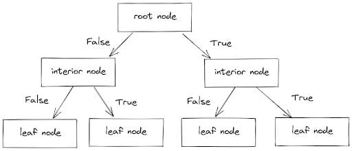
On this part, we’ll take a look at the Resolution Tree Classifier, a machine studying method that’s generally used for classification issues and typically for regression.
The classifier works by dividing information factors into branches, every of which has an interior node (which features a set of situations) and a leaf node (which has the expected worth).
Following these branches and contemplating the situations (True or False), information factors are separated into the right classes. The method is seen beneath.
Picture by Writer
After we apply a Resolution Tree Classifier, we will alter a number of hyperparameters, like the utmost depth of the tree and the utmost variety of leaf nodes.
For our first try, we’ll restrict the variety of leaf nodes to a few with the intention to make the tree easy and comprehensible.
To start, we’ll create a Resolution Tree Classifier with a most of three leaf nodes. This classifier will then be educated on our coaching information and used to generate predictions on the check information. Lastly, we’ll study the accuracy, precision, and recall metrics to evaluate the efficiency of our restricted Resolution Tree Classifier.
Now let’s implement the Resolution Tree algorithm with sci-kit be taught step-by-step.
First, let’s outline a Resolution Tree Classifier object with a most of three leaf nodes, utilizing the DecisionTreeClassifier() perform from the scikit-learn library.
The random_state parameter is used to make sure that the identical outcomes are produced every time the code is run.
<code>tree_3_leaf = DecisionTreeClassifier(max_leaf_nodes= 3, random_state=2)</code>
Then it’s time to practice the Resolution Tree Classifier on the coaching information (X_train and y_train), utilizing the .match() technique.
<code>tree_3_leaf.match(X_train, y_train)</code>
Subsequent, we make predictions on the check information(X_test) utilizing the educated classifier with the predict technique.
<code>y_predict = tree_3_leaf.predict(X_test)</code>
Right here we print the accuracy rating and classification report of the expected values in comparison with the precise goal values of the check information. We use the accuracy_score() and classification_report() capabilities from the scikit-learn library.
<code>print(accuracy_score(y_test, y_predict))
print(classification_report(y_test, y_predict))</code>
Lastly, we’ll plot the confusion matrix to visualise the efficiency of the Resolution Tree Classifier on the check information. We use the plot_confusion_matrix() perform from the scikit-learn library.
<code>fig, ax = plt.subplots(figsize=(12, 9))
plot_confusion_matrix(tree_3_leaf, X_test, y_test, cmap='cividis', ax=ax)</code>
Right here is the code.
<code># Instantiate Resolution Tree Classifier with max leaf nodes = 3
tree_3_leaf = DecisionTreeClassifier(max_leaf_nodes= 3, random_state=2)
# Practice the classifier on the coaching information
tree_3_leaf.match(X_train, y_train)
# Predict the check information with educated tree classifier
y_predict = tree_3_leaf.predict(X_test)
# Print accuracy and classification report on check information
print(accuracy_score(y_test, y_predict))
print(classification_report(y_test, y_predict))
# Plot confusion matrix on check information
fig, ax = plt.subplots(figsize=(12, 9))
plot_confusion_matrix(tree_3_leaf, X_test, y_test, cmap ='cividis', ax=ax)</code>
Right here is the output.

It may be clearly seen from the output, our Resolution Tree works properly, particularly making an allowance for that we restricted it to a few leaf nodes. One of many benefits of getting a easy classifier is that the choice tree might be visualized and comprehensible.
Now, to know how the choice tree makes choices, let’s visualize the choice tree classifier through the use of the plot_tree technique from sklearn.tree.
Right here is the code.
<code>fig, ax = plt.subplots(figsize=(12, 9))
plot_tree(tree_3_leaf, ax= ax)
plt.present()</code>
Right here is the output.
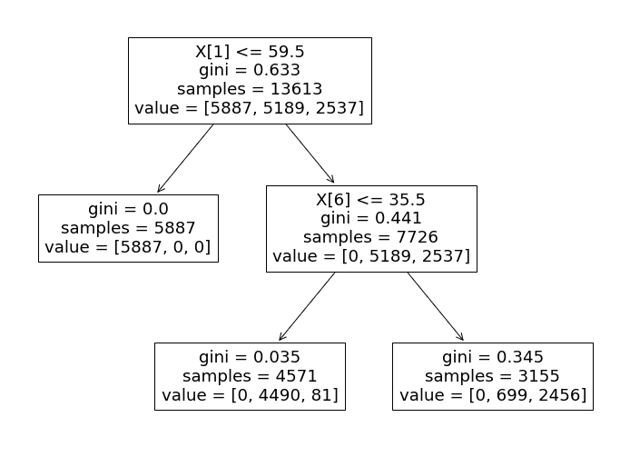
Now let’s analyze this determination tree, and learn the way it carries out the decision-making course of.
Particularly, the algorithm makes use of the ‘tomatometer_rating’ function as the first determinant of every check information level’s classification.
- If the ‘tomatometer_rating’ is lower than or equal to 59.5, the info level is assigned a label of 0 (‘Rotten’). In any other case, the classifier progresses to the subsequent department.
- Within the second department, the classifier makes use of the ‘tomatometer_fresh_critics_count’ function to categorise the remaining information factors.
- If the worth of this function is lower than or equal to 35.5, the info level is labeled as 1 (‘Recent’).
- If not, it’s labeled as 2 (‘Licensed-Recent’).
This decision-making course of intently aligns with the principles and standards that Rotten Tomatoes use to assign film statuses.
In line with the Rotten Tomatoes web site, films are categorised as
- ‘Recent’ if their tomatometer_rating is 60% or increased.
- ‘Rotten’ if it falls beneath 60%.
Our Resolution Tree Classifier follows an analogous logic, classifying films as ‘Rotten’ if their tomatometer_rating is beneath 59.5 and ‘Recent’ in any other case.
Nevertheless, when distinguishing between ‘Recent’ and ‘Licensed-Recent’ films, the classifier should think about a number of extra options.
In line with Rotten Tomatoes, movies should meet particular standards to be categorised as ‘Licensed-Recent’, equivalent to:
- Having a constant Tomatometer rating of at the least 75%
- A minimum of 5 evaluations from prime critics.
- Minimal of 80 evaluations for wide-release movies.
Our restricted Resolution Tree mannequin solely takes into consideration the variety of evaluations from prime critics to distinguish between ‘Recent’ and ‘Licensed-Recent’ films.
Now, we perceive the logic behind the Resolution Tree. So to extend its efficiency, let’s observe the identical steps however this time, we is not going to add the max-leaf nodes argument.
Right here is the step-by-step rationalization of our code. This time I will not broaden the code an excessive amount of as we did earlier than.
Outline the choice tree classifier.
<code>tree = DecisionTreeClassifier(random_state=2)</code>
Practice the classifier on the coaching information.
<code>tree.match(X_train, y_train)</code>
Predict the check information with a educated tree classifier.
<code>y_predict = tree.predict(X_test)</code>
Print the accuracy and classification report.
<code>print(accuracy_score(y_test, y_predict))
print(classification_report(y_test, y_predict))</code>
Plot confusion matrix.
<code>fig, ax = plt.subplots(figsize=(12, 9))
plot_confusion_matrix(tree, X_test, y_test, cmap ='cividis', ax=ax)</code>
Nice now, let’s see them collectively.
This is the entire code.
<code>fig, ax = plt.subplots(figsize=(12, 9))
# Instantiate Resolution Tree Classifier with default hyperparameter settings
tree = DecisionTreeClassifier(random_state=2)

# Practice the classifier on the coaching information
tree.match(X_train, y_train)

# Predict the check information with educated tree classifier
y_predict = tree.predict(X_test)

# Print accuracy and classification report on check information
print(accuracy_score(y_test, y_predict))
print(classification_report(y_test, y_predict))

# Plot confusion matrix on check information
fig, ax = plt.subplots(figsize=(12, 9))
plot_confusion_matrix(tree, X_test, y_test, cmap ='cividis', ax=ax)</code>
Right here is the output.
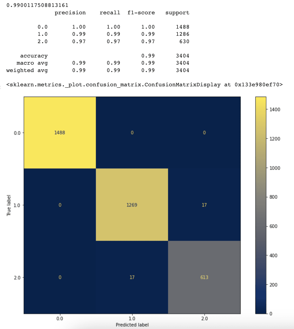
The accuracy, precision, and recall values of our classifier have elevated because of eradicating the utmost leaf nodes limitation. The classifier now reaches 99% accuracy, up from 94% beforehand.
This shows that once we enable our classifier to select the optimum variety of leaf nodes by itself, it performs higher.
Though the present end result seems to be excellent, extra tuning to succeed in even higher accuracy remains to be potential. Within the subsequent half, we’ll look into this feature.
Random Forest Classifier
Random Forest is an ensemble of Resolution Tree Classifiers which were mixed right into a single algorithm. It makes use of a bagging technique to coach every Resolution Tree, which incorporates randomly choosing coaching information factors. Every tree is educated on a separate subset of the coaching information because of this method.
The bagging technique has turn out to be identified for utilizing a bootstrap methodology to pattern information factors, permitting the identical information level to be picked for a number of Resolution Bushes.

Picture by Writer
By utilizing scikit be taught, it’s very easy to use a Random forest classifier.
Utilizing Scikit-learn to arrange the Random Forest algorithm is a straightforward course of.
The algorithm’s efficiency, just like the efficiency of the Resolution Tree Classifier, could also be elevated via altering hyperparameter values such because the variety of Resolution Tree Classifiers, most leaf nodes, and most tree depth.
We are going to use default choices right here first.
Let’s see the code step-by-step once more.
First, let’s instantiate a Random Forest Classifier object utilizing the RandomForestClassifier() perform from the scikit-learn library, with a random_state parameter set to 2 for reproducibility.
<code>rf = RandomForestClassifier(random_state=2)</code>
Then, practice the Random Forest Classifier on the coaching information (X_train and y_train), utilizing the .match() technique.
Subsequent, use the educated classifier to make predictions on the check information (X_test), utilizing the .predict() technique.
<code>y_predict = rf.predict(X_test)</code>
Then, print the accuracy rating and classification report of the expected values in comparison with the precise goal values of the check information.
We use the accuracy_score() and classification_report() capabilities from the scikit-learn library once more.
<code>print(accuracy_score(y_test, y_predict))
print(classification_report(y_test, y_predict))
</code>
Lastly, let’s plot a confusion matrix to visualise the efficiency of the Random Forest Classifier on the check information. We use the plot_confusion_matrix() perform from the scikit-learn library.
<code>fig, ax = plt.subplots(figsize=(12, 9))
plot_confusion_matrix(rf, X_test, y_test, cmap ='cividis', ax=ax)</code>
Right here is the entire code.
<code># Instantiate Random Forest Classifier
rf = RandomForestClassifier(random_state=2)

# Practice Random Forest Classifier on coaching information
rf.match(X_train, y_train)

# Predict check information with educated mannequin
y_predict = rf.predict(X_test)

# Print accuracy rating and classification report
print(accuracy_score(y_test, y_predict))
print(classification_report(y_test, y_predict))

# Plot confusion matrix
fig, ax = plt.subplots(figsize=(12, 9))
plot_confusion_matrix(rf, X_test, y_test, cmap ='cividis', ax=ax)</code>
Right here is the output.

The accuracy and confusion matrix outcomes present that the Random Forest algorithm outperforms the Resolution Tree Classifier. This reveals the benefit of ensemble approaches equivalent to Random Forest over particular person classification algorithms.
Moreover, tree-based machine studying strategies enable us to determine the importance of every function as soon as the mannequin has been educated. For that reason, Scikit-learn supplies the feature_importances_ perform.
Nice, as soon as once more, let’s see the code step-by-step to know it.
First, the feature_importances_ attribute of the Random Forest Classifier object is used to acquire the significance rating of every function within the dataset.
The significance rating signifies how a lot every function contributes to the prediction efficiency of the mannequin.
<code># Get the function significance
feature_importance = rf.feature_importances_</code>
Subsequent, the function importances are printed out in descending order of significance, together with their corresponding function names.
<code># Print function significance
for i, function in enumerate(X_train.columns):
    print(f'{function} = {feature_importance[i]}')</code>
Then to visualise options from an important to least necessary, let’s use argsort() technique from the numpy.
<code># Visualize function from an important to the least necessary
indices = np.argsort(feature_importance)</code>
Lastly, a horizontal bar chart is created to visualise the function importances, with options ranked from most to least necessary on the y-axis and the corresponding significance scores on the x-axis.
This chart permits us to simply determine an important options within the dataset and to find out which options have the best influence on the mannequin’s efficiency.
<code>plt.determine(figsize=(12,9))
plt.title('Characteristic Importances')
plt.barh(vary(len(indices)), feature_importance[indices], colour="b", align='middle')
plt.yticks(vary(len(indices)), [X_train.columns[i] for i in indices])
plt.xlabel('Relative Significance')
plt.present()</code>
Right here is the entire code.
<code># Get the fature significance
feature_importance = rf.feature_importances_

# Print function significance
for i, function in enumerate(X_train.columns):
    print(f'{function} = {feature_importance[i]}')

# Visualize function from an important to the least necessary
indices = np.argsort(feature_importance)

plt.determine(figsize=(12,9))
plt.title('Characteristic Importances')
plt.barh(vary(len(indices)), feature_importance[indices], colour="b", align='middle')
plt.yticks(vary(len(indices)), [X_train.columns[i] for i in indices])
plt.xlabel('Relative Significance')
plt.present()</code>
Right here is the output.
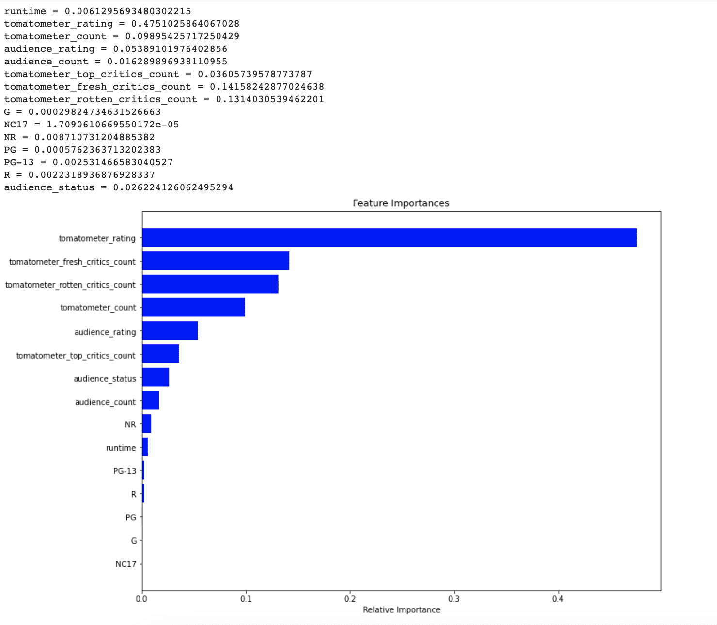
By seeing this graph, it’s clear that NR, PG-13, R, and runtime didn’t think about necessary by the mannequin for predicting unseen information factors. Within the subsequent part, whether or not let’s see addressing this difficulty can improve our mannequin’s efficiency or not.
Random Forest Classifier with Characteristic Choice
Right here is the code.
Within the final part, we found that a few of our options have been thought of much less vital by our Random forest mannequin, in making predictions.
Consequently, to reinforce the mannequin’s efficiency, let’s exclude these much less related options together with NR, runtime, PG-13, R, PG, G, and NC17.
Within the following code, we’ll get the function significance first, then we’ll break up to coach and check set, however contained in the code block we dropped these much less vital options. Then we’ll print out the practice and check set measurement.
Right here is the code.
<code># Get the function significance
feature_importance = rf.feature_importances_
X_train, X_test, y_train, y_test = train_test_split(df_feature.drop(['tomatometer_status', 'NR', 'runtime', 'PG-13', 'R', 'PG','G', 'NC17'], axis=1),df_feature.tomatometer_status, test_size= 0.2, random_state=42)
print(f'Measurement of coaching information is {len(X_train)} and the dimensions of check information is {len(X_test)}')</code>
Right here is the output.

Nice, since we dropped these much less vital options, let’s see whether or not our efficiency elevated or not.
As a result of we did this too many instances, I shortly clarify the next codes.
Within the following code, we first initialize a random forest classifier after which practice the random forest on the coaching information.
<code>rf = RandomForestClassifier(random_state=2)

rf.match(X_train, y_train)</code>
Then we calculate the accuracy rating and classification report through the use of check information and print them out.
<code>print(accuracy_score(y_test, y_predict))
print(classification_report(y_test, y_predict))</code>
Lastly, we plot the confusion matrix.
<code>fig, ax = plt.subplots(figsize=(12, 9))
plot_confusion_matrix(rf, X_test, y_test, cmap ='cividis', ax=ax)</code>
Right here is the entire code.
<code># Initialize Random Forest class
rf = RandomForestClassifier(random_state=2)

# Practice Random Forest on the coaching information after function choice
rf.match(X_train, y_train)

# Predict the educated mannequin on the check information after function choice
y_predict = rf.predict(X_test)

# Print the accuracy rating and the classification report
print(accuracy_score(y_test, y_predict))
print(classification_report(y_test, y_predict))

# Plot the confusion matrix
fig, ax = plt.subplots(figsize=(12, 9))
plot_confusion_matrix(rf, X_test, y_test, cmap ='cividis', ax=ax)</code>
Right here is the output.
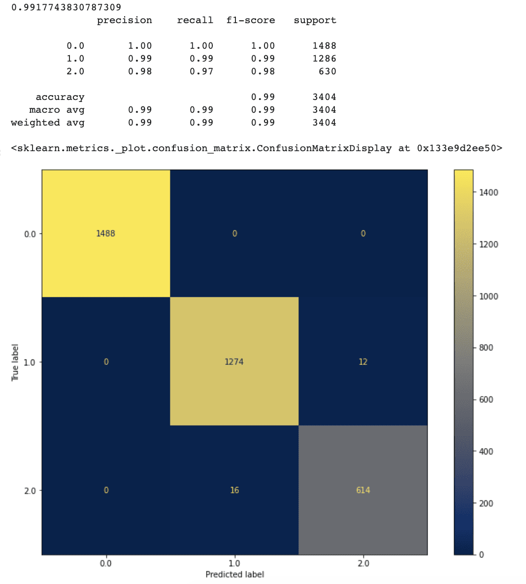
It seems to be like our new method works fairly properly.
After doing function choice, accuracy has elevated to 99.1 %.
Our mannequin’s false optimistic and false adverse charges have additionally lowered marginally when in comparison with the prior mannequin.
This means that having extra traits doesn’t all the time indicate a greater mannequin. Some insignificant traits might create noise which could be the rationale for decreasing the mannequin’s prediction accuracy.
Now since our mannequin’s efficiency has elevated that far, let’s uncover different strategies to examine if we will improve extra.
Weighted Random Forest Classifier with Characteristic Choice
Within the first part, we realized that our options have been a bit imbalanced. Now we have three completely different values, Rotten’ (represented by 0), ‘Recent’ (represented by 1), and ‘Licensed-Recent’ (represented by 2).
First, let’s see the distribution of our options.
This is the code for visualizing the label distribution.
<code>ax = df_feature.tomatometer_status.value_counts().plot(variety='bar', figsize=(12,9))
ax.bar_label(ax.containers[0])</code>
Right here is the output.
It’s clear that the quantity of information with the ‘Licensed Recent’ function is far lower than the others.
To unravel the difficulty of information imbalance, we will use approaches such because the SMOTE algorithm to oversample the minority class or present class weight data to the mannequin throughout the coaching section.
Right here we’ll use the second method.
To compute class weight, we’ll use the compute_class_weight() perform from the scikit-learn library.
Inside this perform, the class_weight parameter is ready to ‘balanced’ to account for imbalanced lessons, and the lessons parameter is ready to the distinctive values within the tomatometer_status column of df_feature.
The y parameter is ready to the values of the tomatometer_status column in df_feature.
<code>class_weight = compute_class_weight(class_weight="balanced", lessons= np.distinctive(df_feature.tomatometer_status),
                      y = df_feature.tomatometer_status.values)</code>
Then, the dictionary is created to map the category weights to their respective indices.
That is accomplished by changing the category weight record to a dictionary utilizing the dict() perform and zip() perform.
The vary() perform is used to generate a sequence of integers comparable to the size of the category weight record, which is then used because the keys for the dictionary.
<code>class_weight_dict = dict(zip(vary(len(class_weight.tolist())), class_weight.tolist()</code>
Lastly, let’s see our dictionary.
Right here is the entire code.
<code>class_weight = compute_class_weight(class_weight="balanced", lessons= np.distinctive(df_feature.tomatometer_status),
                      y = df_feature.tomatometer_status.values)

class_weight_dict = dict(zip(vary(len(class_weight.tolist())), class_weight.tolist()))
class_weight_dict</code>
Right here is the output.

Class 0 (‘Rotten’) has the least weight, whereas class 2 (‘Licensed-Recent’) has the best weight.
After we apply our Random Forest classifier, we will now embody this weight data as an argument.
The remaining code is identical as we did earlier many instances.
Let’s construct a brand new Random Forest mannequin with class weight information, practice it on the coaching set, predict the check information, and show the accuracy rating and confusion matrix.
Right here is the code.
<code># Initialize Random Forest mannequin with weight data
rf_weighted = RandomForestClassifier(random_state=2, class_weight=class_weight_dict)

# Practice the mannequin on the coaching information
rf_weighted.match(X_train, y_train)

# Predict the check information with the educated mannequin
y_predict = rf_weighted.predict(X_test)

#Print accuracy rating and classification report
print(accuracy_score(y_test, y_predict))
print(classification_report(y_test, y_predict))

#Plot confusion matrix
fig, ax = plt.subplots(figsize=(12, 9))
plot_confusion_matrix(rf_weighted, X_test, y_test, cmap ='cividis', ax=ax)</code>
Right here is the output.

Our mannequin’s efficiency elevated once we added class weights, and it now has an accuracy of 99.2%.
The variety of right predictions for the “Recent “ label additionally elevated by one.
Utilizing class weights to handle the info imbalance downside is a helpful technique because it encourages our mannequin to pay extra consideration to labels with increased weights all through the coaching section.
Hyperlink to this information science mission: https://platform.stratascratch.com/data-projects/rotten-tomatoes-movies-rating-prediction
Nate Rosidi is a knowledge scientist and in product technique. He is additionally an adjunct professor educating analytics, and is the founding father of StrataScratch, a platform serving to information scientists put together for his or her interviews with actual interview questions from prime corporations. Join with him on Twitter: StrataScratch or LinkedIn.


