Is chatgpt good at generating code for tuning a guitar ?

Science he was a patented CS engineer he wanted to prove me that my new guitar tuner was useless since AI could come with a better less convoluted exact example in less lines of code than mine (mine is adapted from a blog on audio processing and fast fourier transform because it was commented and was refreshing me the basics of signal processing).
And I asked him, have you ever heard of the Nyquist frequency ? or the tradeoff an oscilloscope have to do between time locality and accuracy ?
Of course he didn’t. And was proud that a wannabee coder would be proven useless thanks to the dumbest AI.
So I actually made this guitar tuner because this time I wanted to have an exact figure around the Hertz.
The problem stated by FFT/Nyquist formula is that if I want an exact number around 1Hz (1 period per second) I should sample at least half a period (hence .5 second), and should not expect a good resolution.
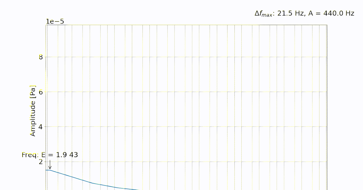
The quoted chatgpt code takes 1024 samples out of 44100/sec, giving it a nice reactivity of 1/44th of a second with an accuracy of 44100/1024/2 => 21Hz.
I know chatgpt does not tune a guitar, but shouldn’t the chatgpt user bragging about the superiority of pro as him remember that when we tune we may tune not only at A = 440Hz but maybe A = 432Hz or other ?
A note is defined as a racine 12th of 2 compared to an arbitrary reference (remember an octave is doubling => 12 half tones = 2) ; what makes a temperate scale is not the reference but the relationship between notes and this enable bands of instrument to tune themselves according to the most unreliable but also nice instrument which is the human voice.
Giving the user 3 decimal after the comma is called being precise : it makes you look like a genius in the eye of the crowd. Giving the user 0 decimal but accurate frequency is what makes you look dumb in the eyes of the computer science engineer, but it way more useful in real life.
Here I took the liberty with pysine to generate A on 6 octaves (ref A=440) and use the recommanded chatgpt buffer size acknowledged by a pro CS engineer for tuning your guitar and my default choices.
for i in 55.0 110.0 220.0 440.0 880.0 1760.0 ; do python -m pysine $i 3; done
Here is the result with a chunk size of 1024 :
And here is the result with a chunk size corresponding to half a second of sampling :

I may not be a computer engineer, I am dumb, but checking with easy to use tools that your final result is in sync with your goal is for me more important than diplomas and professional formations.
The code is yet another basic animation in matplotlib with a nice arrow pointing the frequency best fitting item. It is not the best algorithm, but it does the job.
Showing the harmonics as well as the tonal has another benefit it answers the questions : why would I tune my string on the note of the upper string ?
Like tuning E on A ?
Well because –at least for my half broken guitar– it ensures to me that I will tune on the tonal note.
Here is a sample of tuning E on the empty string :

And this is how tuning the E string on the A note looks like :

And don’t pay attention to the 56Hz residual noise triggered by my fans/appliance turning and making a constant noise 😀
Here is the code
import pyaudio
import matplotlib.pyplot as plt
import matplotlib.animation as animation
import numpy as np
import time
from sys import argv

A = 440.0
try:
    A=float(argv[1])
except IndexError:
    pass

form_1 = pyaudio.paInt16 # 16-bit resolution
chans = 1 # 1 channel
samp_rate = 44100 # 44.1kHz sampling rate
chunk = 44100//2# .5 seconds of sampling for 1Hz accuracy

audio = pyaudio.PyAudio() # create pyaudio instantiation

# create pyaudio stream
stream = audio.open(
    format = form_1,rate = samp_rate,channels = chans,
    input = True , frames_per_buffer=chunk
)

fig = plt.figure(figsize=(13,8))
ax = fig.add_subplot(111)
plt.grid(True)
def compute_freq(ref, half_tones):
    return [ 1.0*ref*(2**((half_tones+12*i )/12)) for i in range(-4,4)   ]

print(compute_freq(A,0))
note_2_freq = dict(
    E = compute_freq(A,-5),
    A = compute_freq(A, 0),
    D = compute_freq(A, 5),
    G = compute_freq(A,-2),
    B = compute_freq(A, 2),
    )
resolution = samp_rate/(2*chunk)

def closest_to(freq):
    res = dict()
    for note, freqs in note_2_freq.items():
        res[note]=max(freqs)
        for f in freqs:
            res[note]= min(res[note], abs(freq -f))
    note,diff_freq = sorted(res.items(), key = lambda item : item[1])[0]

    for f in note_2_freq[note]:
        if abs(freq-f) == diff_freq:
            return "%s %s %2.1f %d" % (
                note,
                abs(freq - f ) < resolution and "=" or
                    ( freq > f and "+" or "-"),
                abs(freq-f),
                freq
            )

def init_func():
    plt.rcParams['font.size']=18
    plt.xlabel('Frequency [Hz]')
    plt.ylabel('Amplitude [Arbitry Unit]')
    plt.grid(True)
    ax.set_xscale('log')
    ax.set_yscale('log')
    ax.set_xticks( note_2_freq["E"] + note_2_freq["A"]+
                  note_2_freq["D"]+ note_2_freq["G"]+
                  note_2_freq["B"] ,
                labels = (
                    [ "E" ] * len(note_2_freq["E"]) +
                    [ "A" ] * len(note_2_freq["A"]) +
                    [ "D" ] * len(note_2_freq["D"]) +
                    [ "G" ] * len(note_2_freq["G"]) +
                    [ "B" ] * len(note_2_freq["B"])
                    )
    )

    ax.set_xlim(40, 4000)
    return ax

def data_gen():
    stream.start_stream()
    data = np.frombuffer(stream.read(chunk),dtype=np.int16)
    stream.stop_stream()
    yield data
i=0
def animate(data):
    global i
    i+=1
    ax.cla()
    init_func()
    # compute FFT parameters
    f_vec = samp_rate*np.arange(chunk/2)/chunk # frequency vector based on window
                                               # size and sample rate
    mic_low_freq = 50 # low frequency response of the mic
    low_freq_loc = np.argmin(np.abs(f_vec-mic_low_freq))
    fft_data = (np.abs(np.fft.fft(data))[0:int(np.floor(chunk/2))])/chunk
    fft_data[1:] = 2*fft_data[1:]
    plt.plot(f_vec,fft_data)

    max_loc = np.argmax(fft_data[low_freq_loc:])+low_freq_loc

# max frequency resolution
    plt.annotate(r'$\Delta f_{max}$: %2.1f Hz, A = %2.1f Hz' % (
            resolution, A), xy=(0.7,0.92), xycoords="figure fraction"
    )
    ax.set_ylim([0,2*np.max(fft_data)])

    # annotate peak frequency
    annot = ax.annotate(
        'Freq: %s'%(closest_to(f_vec[max_loc])),
        xy=(f_vec[max_loc], fft_data[max_loc]),\
        xycoords="data", xytext=(0,30), textcoords="offset points",
        arrowprops=dict(arrowstyle="->"),
        ha="center",va="bottom")
    #fig.savefig('full_figure-%04d.png' % i)
    return ax,

ani = animation.FuncAnimation(
    fig, animate, data_gen, init_func, interval=.15,
    cache_frame_data=False, repeat=True, blit=False
)
plt.show()


